✏️ Book Problems (Chapter 6)

Question 1

This question is in the textbook, but I see some problems in it. Do you see them, too?

✏️ Which of the following choices best completes the following statement? Explain.

An investor with a higher degree of risk aversion, compared to one with a lower degree, will demand investment portfolios …

1. with higher risk premiums.
2. that are riskier (with higher standard deviations).
3. with lower Sharpe ratios.
4. with higher Sharpe ratios.

✔ Click here to view answer

D.

They would demand a point that is “lower” on the CAL - ie y, σ, and E(r_C) would be lower.

Clearly, a and b can’t be correct because a more risk averse person would choose a point on the CAL with lower risk premium (because they would choose a point with lower E(r_C) and with less risk.)

However all investors would always choose a higher Sharpe ratio. That’s clearly the best option. I don’t like this question, though because a person with higher risk aversion isn’t more likely to do this.

Question 2

✏️ Which of the following statements are true? Explain.

1. A lower allocation to the risky portfolio reduces the Sharpe (reward-to-volatility) ratio.
2. The higher the borrowing rate, the lower the Sharpe ratios of levered portfolios.
3. With a fixed risk-free rate, doubling the expected return and standard deviation of the risky portfolio will double the Sharpe ratio.
4. Holding constant the risk premium of the risky portfolio, a higher risk-free rate will increase the Sharpe ratio of investments with a positive allocation to the risky asset.

✔ Click here to view answer

Changing the allocation to the risky portfolio doesn’t change the Sharpe ratio at all, so A is wrong.

B is correct - it is referring to the “kinked CAL” that Bruce covered in class. The borrowing rate is the interest rate when you borrow money so that you can invest more than 100% of your assets in the risky portfolio (ie y > 0).

We always assume that the borrowing rate is at least as high as the risk free rate because lending to investors implies risk and riskier investments require a higher return. This higher borrowing rate “kinks” the CAL downward, lowering the Sharpe ratio.

Question 5

✏️ Consider a portfolio that offers an expected rate of return of 7% and a standard deviation of 18%. T-bills offer a risk-free 2% rate of return. What is the maximum level of risk aversion for which the risky portfolio is still preferred to T-bills?

✔ Click here to view answer

We will assume that the investor must choose either one asset or another and that they can’t choose a mix.

Because this refers to the “level of risk aversion,” it expects us to use $U = E(r)- \tfrac{1}{2}Aσ^2$
Utility of the risky portfolio:

$$U = E(r)- \tfrac{1}{2}Aσ^2 = 7\%- \tfrac{1}{2}A ×18\%^2$$

Utility of the riskless asset:

$$U = E(r)- \tfrac{1}{2}Aσ^2 = 2\%$$

What is the maximum level of risk aversion for which:

$$U(\text{risky}) > U(r_F)$$

$7\%-\tfrac{1}{2}A×18\%^2 >2\%$
$-\tfrac{1}{2}A×18\%^2 >2\%-7\%$
$-\tfrac{1}{2}A×18\%^2 >-5\%$
$\tfrac{1}{2}A×18\%^2 < 5\%$
$A < \frac{5\%}{\tfrac{1}{2}18\%^2} = 3.0864$

As long as A < 3.0864, the investor will prefer the risky portfolio. If A> 3.0864, they will prefer the risk-free asset. (We’re assuming that they can only choose one.)

Status

We could try these some time if people liked. They are relevant to this class, but only barely so. Email me if you’d like us to cover these questions in section. robecon1452@gmail.com

6. ✏️Draw the indifference curve in the expected return-standard deviation plane corresponding to a utility level of .02 for an investor with a risk aversion coefficient of 3. (Hint: Choose several possible standard deviations, ranging from 0 to .25, and find the expected rates of return providing a utility level of .02. Then plot the expected return-standard deviation points so derived.)
7. ✏️ Now draw the indifference curve corresponding to a utility level of .02 for an investor with risk aversion coefficient A = 4. Comparing your answer to Problem 6, what do you conclude?
8. ✏️ Draw an indifference curve for a risk-neutral investor providing utility level .02.
9. ✏️ What must be true about the sign of the risk aversion coefficient, A, for a risk lover? Draw the indifference curve for a utility level of .02 for a risk lover.

For Problems 10 through 12: Consider historical data showing that the average annual rate of return on the S&P 500 portfolio over the past 95 years has averaged roughly 8% more than the Treasury bill return and that the S&P 500 standard deviation has been about 20% per year. Assume these values are representative of investors’ expectations for future performance and that the current T-bill rate is 2%

Question 10

✏️ Calculate the expected return and variance of portfolios invested in T-bills and the S&P 500 index with weights as follows:

Wbills	Windex
0	1.0
0.2	0.8
0.4	0.6
0.6	0.4
0.8	0.2
1.0	0

✔ Click here to view answer

BKM, Chapter 6, Qs 10 and 11

Question 11

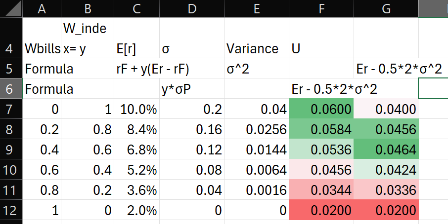
✏️ Calculate the utility levels of each portfolio of Problem 10 for an investor with A = 2. What do you conclude?

✔ Click here to view answer

BKM, Chapter 6, Qs 10 and 11

Question 12

✏️ Repeat Problem 11 for an investor with A = 3. What do you conclude?

✔ Click here to view answer

BKM, Chapter 6, Qs 10 and 11