Big Picture

Return and Risk In Two Equations and a Graph

Investment is a tradeoff between return and risk:

The upside of investing is that we expect to earn a return on our money. We measure this by calculating expected value of our return: $E(r)$ .
The downside of investing is that there is risk. We measure this by calculating the standard deviation of of our return: $σ_C$ .

The most important formulas in this lecture - by far - help us predict these two quantities:

E(r_C) = r_F + y(E(r_P) - r_F)

σ_C = yσ_P

If you understand these two equations, you are well on your way to mastery of the material in this lecture. The equations are vital because they allow us to predict our levels of risk and return based on how we allocate our capital. What we can predict, we can control (at least to some degree).

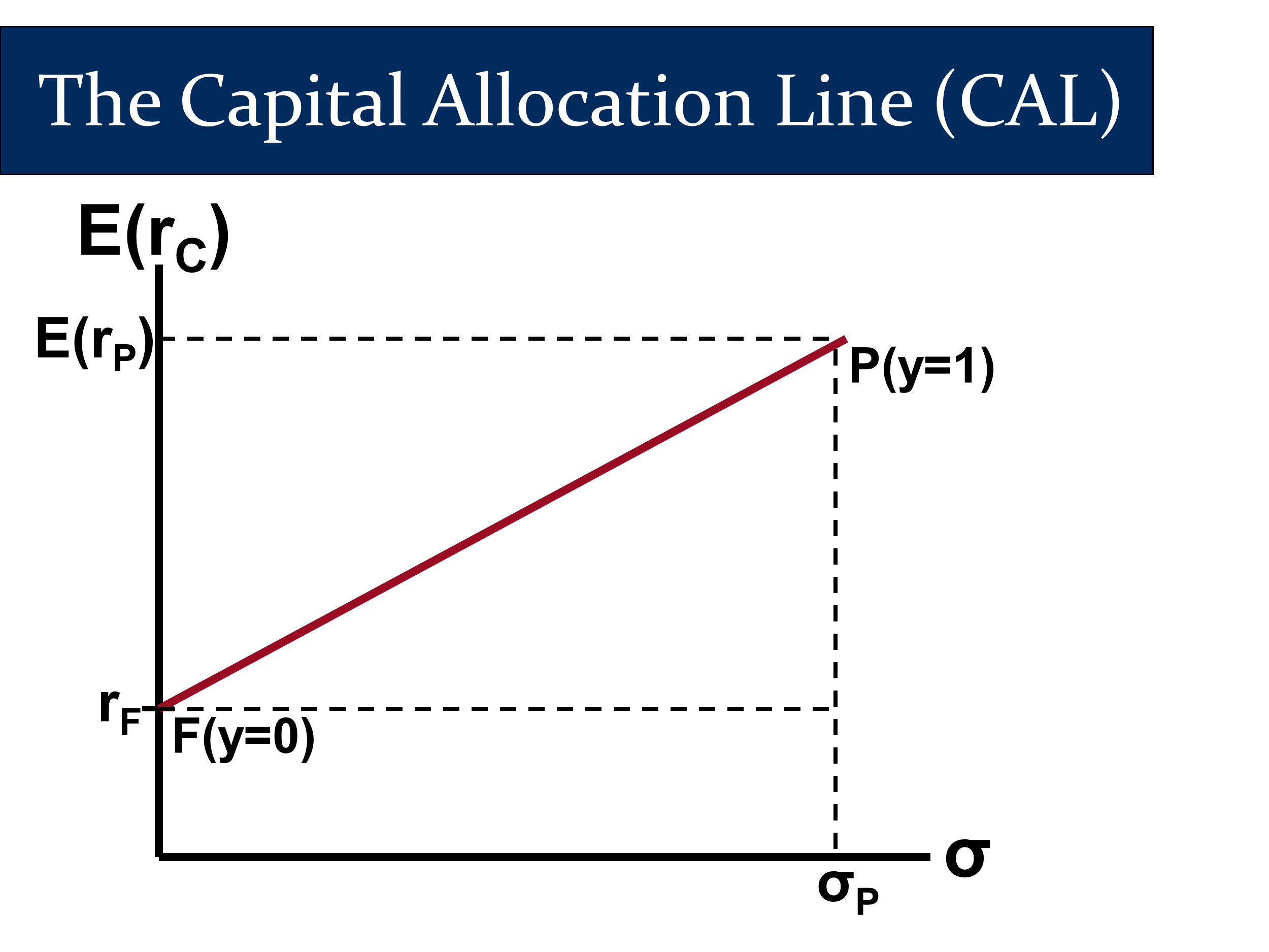
Our key diagram also focuses on the same two quantities. Note that risk/ $σ_C$ is on the horizontal axis and return/ $E(r)$ is on the vertical axis of the following diagram:

Applications

We use the two equations and the graph to see how our expected return and risk are determined by $y$ , the percentage of our wealth that we invest in risky asset. We call this the “Capital Allocation Decision” because we are deciding what percentage of our capital we want to allocate to risky and risk-free assets. That is why we refer to line in our diagram as the “Capital Allocation Line (CAL).”

I like to approach the Capital Allocation Decision by imagining myself as a financial advisor. The CAL is a “menu” of potential complete portfolios that I can offer to my clients. They will choose the complete portfolio that matches their risk tolerances (determined by time to retirement and personality). We will talk more about this later.

We also look at how well we are trading off risk vs return by looking at the ratio of our return to our risk. This is known as the “Reward to Risk Ratio” or the “Sharpe Ratio.” (We subtract off the risk-free rate, $r_F$ , when calculating the “reward” because we only consider returns in excess of the risk-free rate to count as rewards for taking risk.)

That’s it!

That’s it - except for one remaining idea, those are the main ideas from the lecture. We can fill in details with a careful slide review.

For everything you learn in this lecture, try to connect it back to these two concepts - risk/ $σ_C$ and return/ $E(r)$ .

Coming Attractions

Most of this lecture focused on the formulas for risk and return as you varied the amount of a risk-free asset and a risky asset in your portfolio.

But what if you have two risky assets?

With both assets risky, you’ll get new formulas for expected return and risk/standard deviation. Look out for them next lecture.

These new tools will help us understand how to build an optimal portfolio of risky assets. This graph will have a curve in it that illustrates a “free” way to reduce risk

Together, this lecture and the next make up what is known as “Modern Portfolio Theory.” Coming to section and carefully reviewing this lecture’s material will help you appreciate and understand not just this week’s material, but next week’s material also.

Finally, in the lecture after this one, we will apply modern portfolio theory to understand the Capital Asset Pricing Model.

We can understand the risk-return tradeoff by asking how much expected return do we get per unit of risk we take on. This is the Sharpe ratio: The reward to volatility ratio