🔎 Notes on CAPM from e2000

Formulas for this lecture can be found in the formula sheet.

Optimal Diversification

As you add more stocks to your portfolio, the risk in your portfolio, measured as standard deviation (σ), decreases:

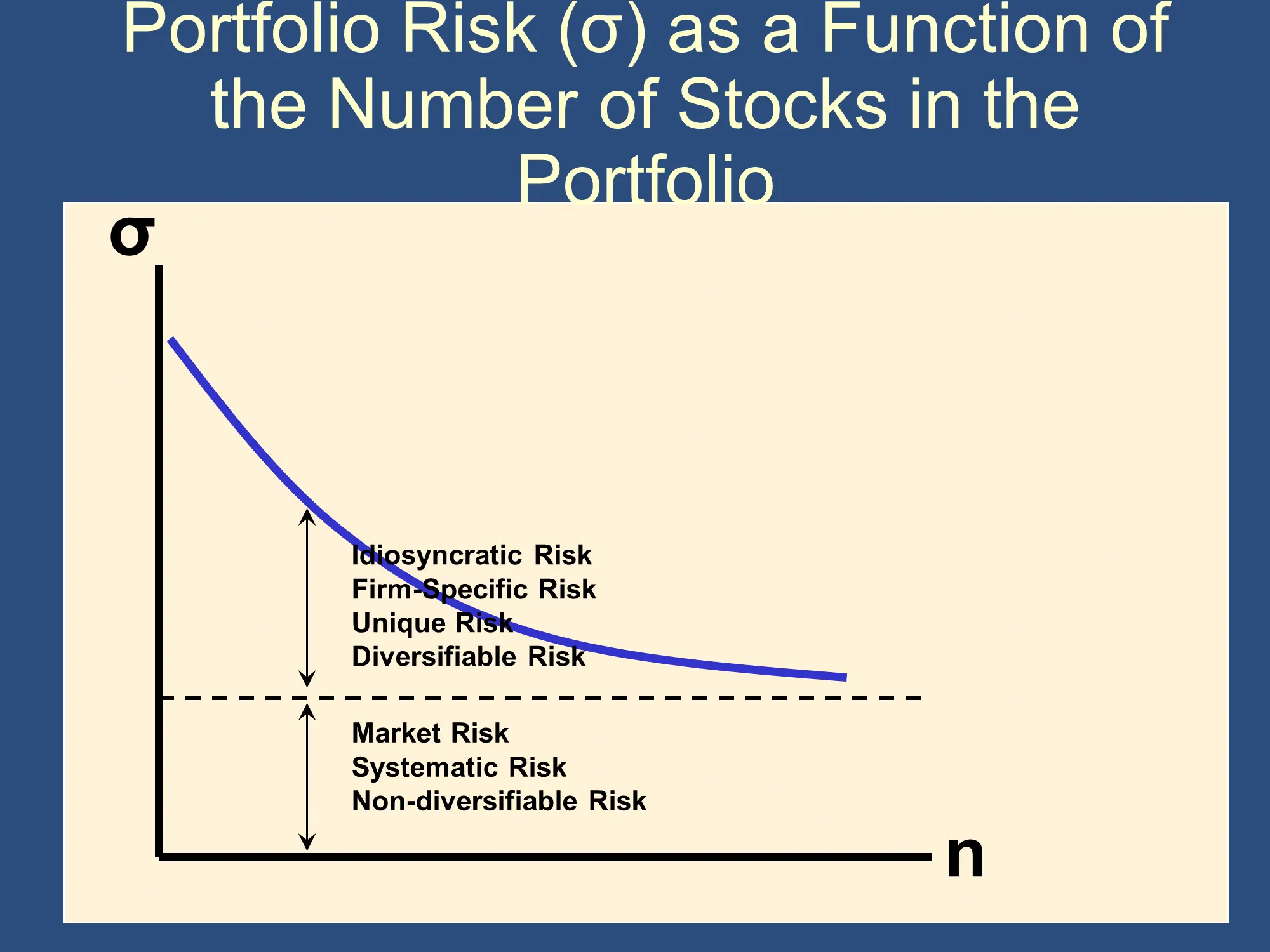However, it doesn’t decrease down to zero. Rather, it approaches a floor level of “market risk.”

This allows us to divide all of the risk in our portfolio into two types:

• Idiosyncratic/Firm-Specific/Diversifiable Risk - with proper diversification, we can remove this risk from our portfolio. The more stocks we add to our portfolio, the more of the idiosyncratic risk we can remove.
• Market/Systematic/Non-diversifiable Risk - this type of risk can’t be “diversified away” by adding more stocks and bonds. Note for later: β is a measure of the market/systematic/non-diversifiable risk of a stock (or of a portfolio of stocks).

It’s pretty amazing that diversification (which is free) can significantly reduce the idiosyncratic risk in your portfolio. How does it do that? Diversification works because if one of your securities “does poorly,” there is a good chance that another security “does well,” and this can lessen the total risk in your portfolio. The good performance of the second security can “dull the pain” from the first security. This is, fundamentally, all that diversification is about.

This explanation assumes that when the first security does poorly, the second security tends to do well, to counterbalance the first. If this is the case, the securities are said to be “negatively correlated,” because the two securities have opposite performances (ie when one has a lower return than it usually has, the other has a higher return than it usually has). Negatively correlated securities provide less diversification, because losses by one security tend to be cancelled out by gains in other securities.

As we’ve seen, negative correlation is good for investors because it allows one security to provide a form of insurance against risk in another security. Unfortunately, negative correlation is fairly rare. In fact, typically, the IRR/return on assets with negative correlation with the market is negative. In other words, rather than earning money when you invest in them, they typically cost you money on average. Just as you must pay for health insurance or car insurance, you must pay for negative correlation.

What is far more common is positive correlation. Diversification still works with positive correlation, but it is not as effective. Security A and Security B are positively correlated if, when Security A does below average, Security B is more likely to also do below average. To see why this leads to poor diversification, imagine you had a considerable amount of money invested in Security A. You are worried about the risk of security A losing money (having a negative return). Therefore, you transfer some of your money from Security A to Security B. This will provide a tiny bit of diversification because if Security A has a low return, Security B might have a high return. However, because they are positively correlated, it is more likely that Security B will also have a low return. For example, suppose you are concerned about a loss of 10% on Security A. If you attempt to diversify to Security B and security B also has a loss of 10%, then your portfolio will still have a loss of 10%. You will have had no benefits of diversification.

This is what Bruce means in the following slide:

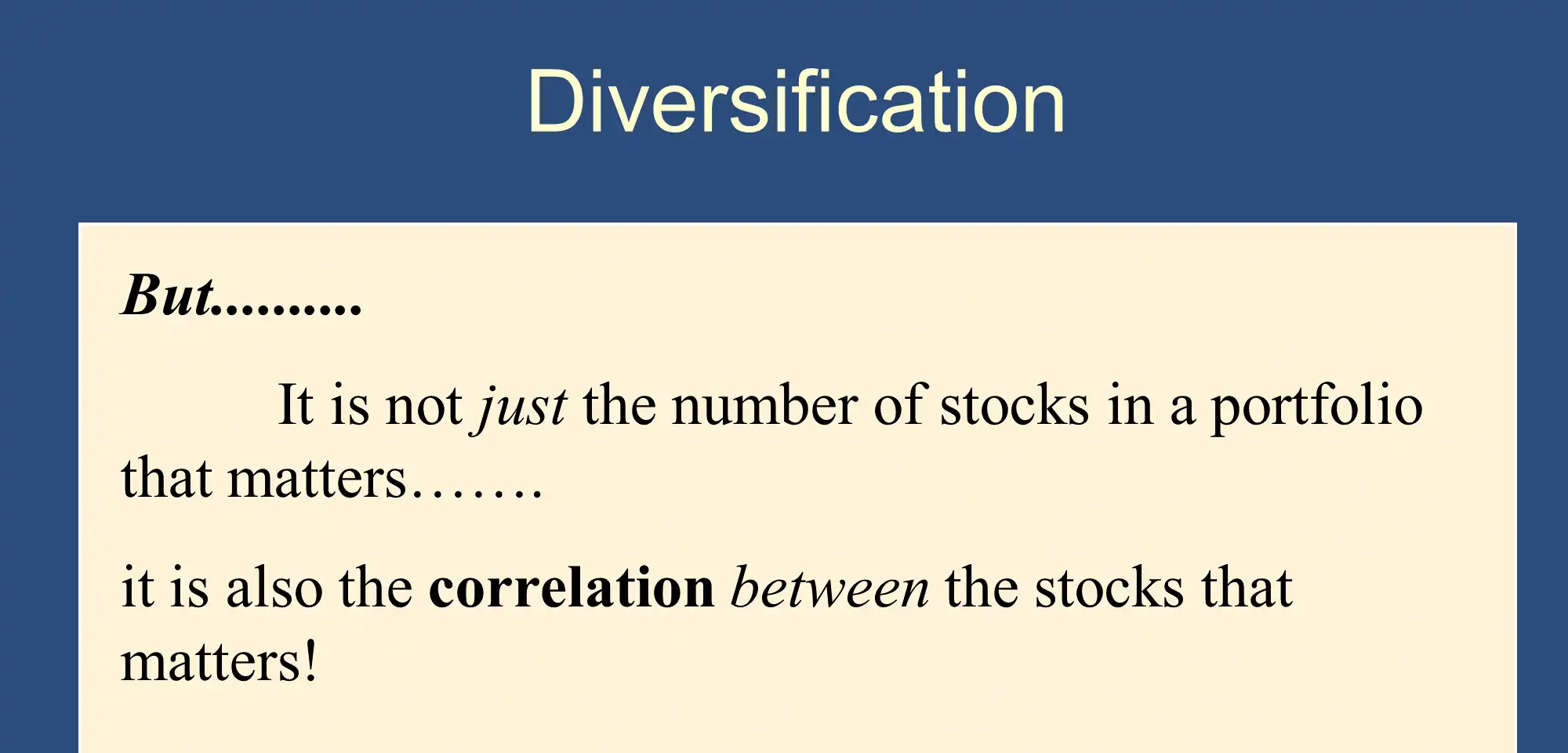
The limits to diversification come from the fact that various securities are typically correlated. Much of the performance of any given stock on any given day can be predicted by how the Dow Jones Average does on that day. If the Dow is down, the vast majority of stocks will also be down. Therefore, diversifying into many, many stocks won’t save you from a day on which the Dow is down. This, fundamentally is what systematic risk is. It’s based on the fact that all securities tend to move together, so they can’t cancel losses out from the other securities as well as we might hope.

The concept of correlation is precisely defined in probability, statistics, data science, advanced finance, and many other courses. It can be calculated from historical data, but you are not responsible for knowing how in this class. However, for reference, here are the correlations between some common stocks and a portfolio with all US stocks:

	Correlation with the VTI ETF
Amazon	59%
IBM	58%
Disney	74%
Microsoft	62%
Boeing	58%
Starbucks	58%
ExxonMobil	59%

Source

When stocks are negatively correlated, the number for mathematical correlation is negative. As you can see the stocks above are quite significantly correlated with the US stock market as a whole.

Ray Dalio breaks down his “Holy Grail”

The Capital Asset Pricing Model (CAPM)

The CAPM is a mathematical model that says that under certain assumptions, the expected returns that investors demand for a stock are determined by the systemic risk (β) that the stocks have.

The CAPM is a mathematical theory that says that there is a tradeoff between risk and higher returns. This is captured in the following formula, where β represents risk and $E(r_S)$ represents the return on a specific Stock. Note that the return in the

$$E(r_S) = r_F+ β[E(r_M) - r_F]$$

There is a formula for beta that can be used to estimate beta using historical data. Intuitively, however, Beta represents a “non-diversifiable risk.”

Investors don’t want to be exposed to risk, and they especially don’t want to be exposed to non-diversifiable risk Within the assumptions of the CAPM, investors can and will diversify away the idiosyncratic risk. Therefore, investors don’t care about idiosyncratic risk - they only care about systematic risk, which is captured in β. This is why β completely determines expected returns in the CAPM.

Side note: To understand the CAPM, you need to understand that the CAPM is a mathematical model much like the money multiplier model is a model. Like the money multiplier model, the CAPM is a useful model that can help us understand why things happen the way that they happen. Like the money multiplier model, the CAPM is based on certain assumptions. Those assumptions are that everyone starts with roughly the same beliefs about the world and that these beliefs are largely true. Likewise, the CAPM assumes that everyone is very sophisticated about diversification and that there are many securities to invest in. It uses the tools of supply and demand and probability theory to investigate what drives securities prices. What does this mean for you? Just know that there is a lot of modeling that has been done, and when similar assumptions are used, similar conclusions are arrived at. We want to get a sense of those assumptions and those conclusions. That’s all we need to do!

Fundamentally, the above equation tells you the expected rate of return that investors will require if they are going to be willing to invest in/hold the security.

Values of Beta:

• For the market as a whole, $β = 1$
• $β>1$ implies stock requires a return greater than the market return, because the stock is riskier (has a higher standard deviation) than the market
• $β<1$ implies stock requires a return lower than the market return, because the stock is less risky (has a lower standard deviation) than the market

The main skill you’ll need to develop is applying the main CAPM formula.

Stock	Beta	$E(r_S)$
Amazon	2.20	20.4%
IBM	1.59	16.1%
Disney	1.26	13.8%
Microsoft	1.13	12.9%
Boeing	1.09	12.6%
Starbucks	.69	9.8%
ExxonMobil	.65	9.6%

Assume that

• the risk-free rate $= r_F = 5\%$
• the expected return on the market portfolio $= E(r_M) = 12\%$ Therefore, the expected risk premium on the market $= E(r_M)-r_F = 12\% - 5\% = 7\%$

The above table says that Amazon has a huge amount of non-diversifiable risk $(β=2.2)$. Therefore, within the CAPM model, investors won’t be willing to own it unless they have an expected return of 20.4% when owning Amazon: $E(r_S) = r_F + β[E(r_M) - r_F] = 5\% + 2.2 \times (12\% - 5\%) = 20.4\%$

✏️ Suppose that that Meta has β=1.3. What is the expected return on Meta, based on the above assumptions.

✔ Click here to view answer

$E(r_S) = r_F + β[E(r_M) - r_F] = 5\% + 1.3 \times (12\% - 5\%) = 14.1\%$

⚠️ This is a potential ‘gotcha’ on the exam.

✏️ Suppose that the risk premium on the market was 9% instead of 7%. What would the expected return on Meta be?

✔ Click here to view answer

Here, we are given $E(r_M)-r_F$, so we just plug it directly into the formula:

$$E(r_S) = r_F + β[E(r_M) - r_F] = 5\% + 1.3 \times 9\% = 16.7\%$$

Whenever you see the phrase, “risk premium” make sure to look the term up in the following Jargon cheat sheet.

Jargon cheat sheet

CAPM Notation	Associated Terminology
$r_F = 5\%$	Risk free rate OR return on T-Bills OR return on short term government securities return on securities perceived to be risk-free
$E(r_S) = 12\%$	Expected (rate of) return offered by a specific stock OR Expected rate of return required by the market for a specific portfolio (or stock) $E(r_i)$ and $E(r_S)$ mean the same thing. ‘i’ just refers to a numbered security and ‘s’ just refers to a specific stock.
$E(r_S) - r_F = 7\%$	(Expected) risk premium for a specific stock Note: I can get 5% by investing in risk-free assets, so I ignore the first 5% of the return from investing in a stock. I’m only interested in the 7% risk premium that I get above the risk-free rate.
$β$	Beta (a measure of non-diversifiable risk)
$r_M$	The actual return on the market portfolio. Note: We imagine a portfolio consisting of every single stock, bond, and other security in existence. We call this special portfolio “the market portfolio.” $r_M$ is the expected return of the market portfolio.
$E(r_M)$	Expected return of the market OR Expected market return OR Expected return of/on the market portfolio
$E(r_M)-r_F$	(Expected) Risk Premium of the market OR (Expected) Risk Premium of the market portfolio

✏️ You are evaluating a risky stock. You expect the stock to have a return of 17%, but because the stock is so risky, you don’t know if it is actually a good investment. You expect the overall market to have a return of 12%. The risk free rate is 2% and the beta for this stock is 2.4. What return would the CAPM expect for this stock? Is it a good investment?

✔ Click here to view answer

$E(r_M)=12\%$, $r_F = 2\%$, $β=2.4$
$E(r_S) = r_F + β[E(r_M) - r_F] = 2\% + 2.4 \times (12\% - 2\%) = 26\%$
The CAPM predicts that this stock is risky enough that it should have a return of 26%. However, your analysis suggests that it will only have a return of 17%. That’s not enough to compensate you for the riskiness of the stock. Therefore, it’s a bad investment.

Applications of the CAPM

• Calculating required rates of return to calculate discount rates.
• Performance evaluation of portfolio managers (calculate the return they should be earning based on the beta of their portfolio and then compare their actual results to that prediction.)
• A way to conceptualize investment decisions and to understand diversification.

Fundamental analysis: Attempt to determine a stock’s fundamental value by analyzing the company, the industry, and the macroeconomy. Technical analysis: looking at stock price charts to find and exploit recurring and predictable patterns