👨‍🏫 Notes

Markowitz Portfolio Optimization

The bulk of this lecture is based on Markowitz Portfolio optimization, which is an process for finding optimal allocations in a portfolio. It was derived from classical tools of probability.

It has three steps:

1. Find the optimal risky portfolio.
2. Build the CAL. The CAL is like a menu of different complete portfolios that an investor may choose, based on their risk aversion.
3. Choose the complete portfolio off of the CAL that matches the investor’s risk preferences.

This entire process is illustrated in the following Excel spreadsheet:

Modern Portfolio Theory

Find the optimal risky portfolio

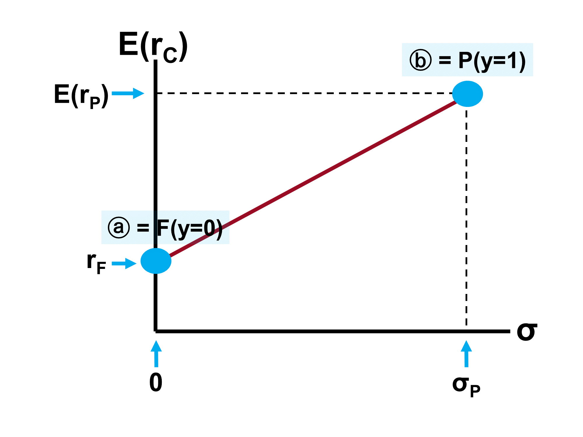
The following slide show a pair of assets. As you can see from the diagram, Asset 1 has a lower σ and Er. Specifically, it looks like $σ_1=12\%$ and $E_{r1}=8\%$, whereas $σ_2=20\%$ and $E_{r2}=13\%$. Therefore, we can think of asset 1 as bonds and asset 2 as stocks.

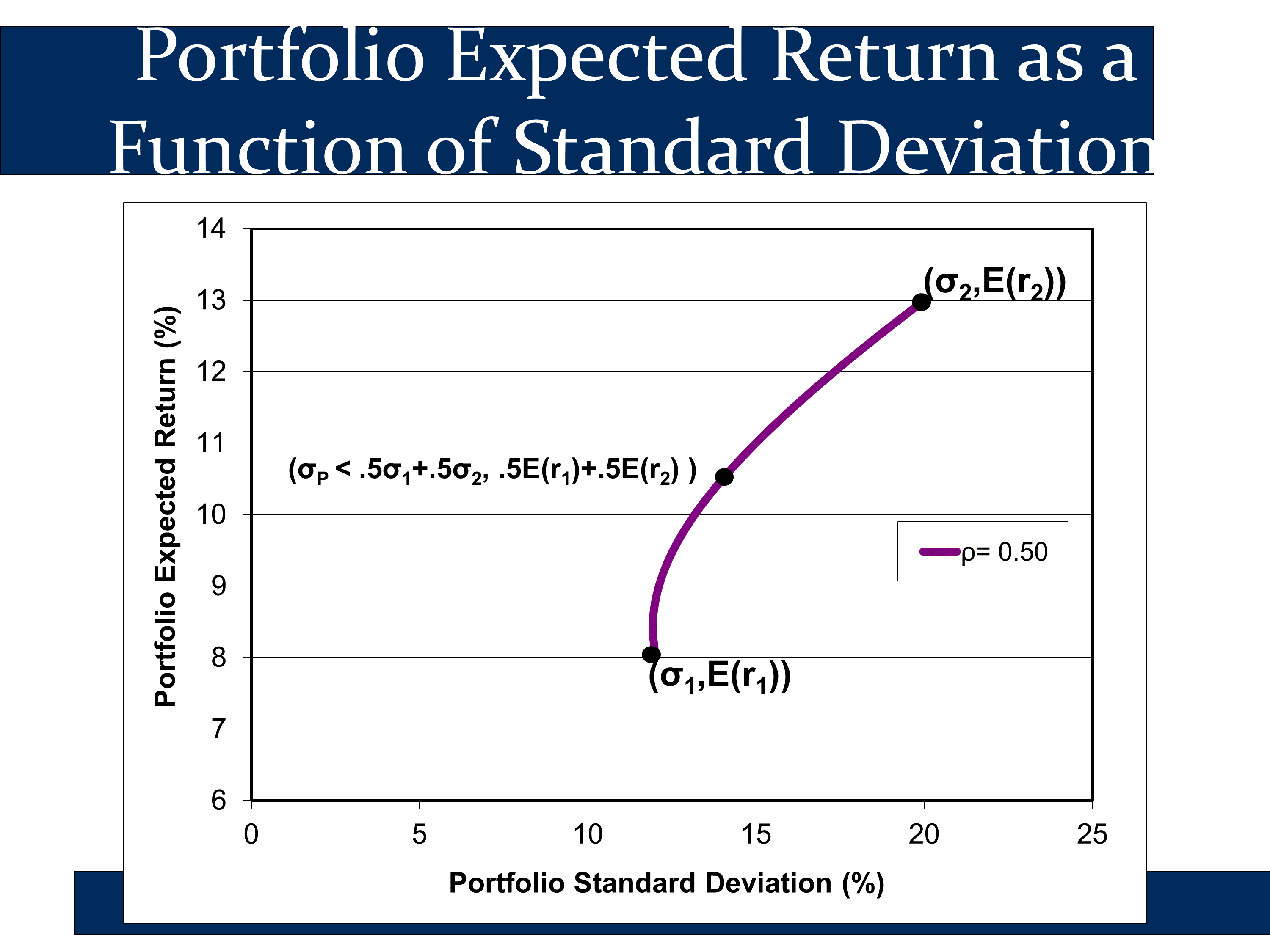
The purple line shows all combinations of assets 1 and 2 that the investor can own. For example, the highest black dot represents a portfolio invested 100% in stock and the lowest black dot represents a portfolio invested 100% in bonds. The other points on the purple line represent all of the other possible weightings of the portfolio.

The middle black point represents a portfolio that is 50% invested in stocks and 50% invested in bonds. This investor puts half of their money in each asset. Note the following label for this portfolio:

The second half of the label indicates that the expected return of the “50/50 portfolio” is a 50/50 weighted average of the expected returns of stocks and bonds:

$$E(r_p) = 50\% × E(r_1) + 50\% × E(r_2)$$

Likewise, the label also indicates that the standard deviation of the 50/50 portfolio is lower than the 50/50 weighted average of the standard deviation:

$$σ_P < .5σ_1 + .5σ_2$$

This is due to the benefits of diversification when the correlation between the assets is less than 1 (which it almost always is).

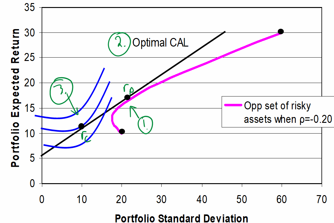
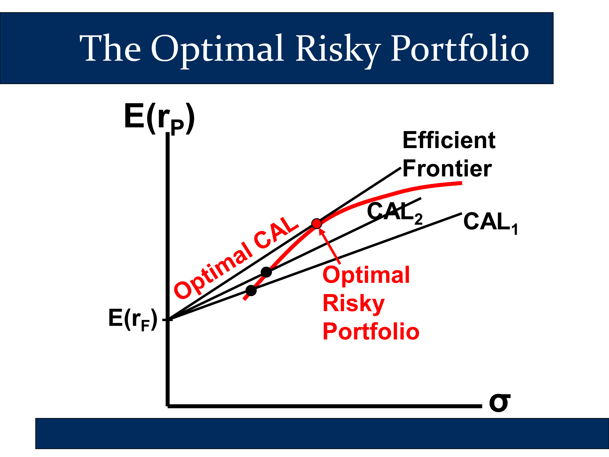
The followings slide indicates that you can get the “best” (=highest return) CAL from the point on the curved line:

1. where the CAL is tangent to the curved line
2. the Sharpe ratio is highest

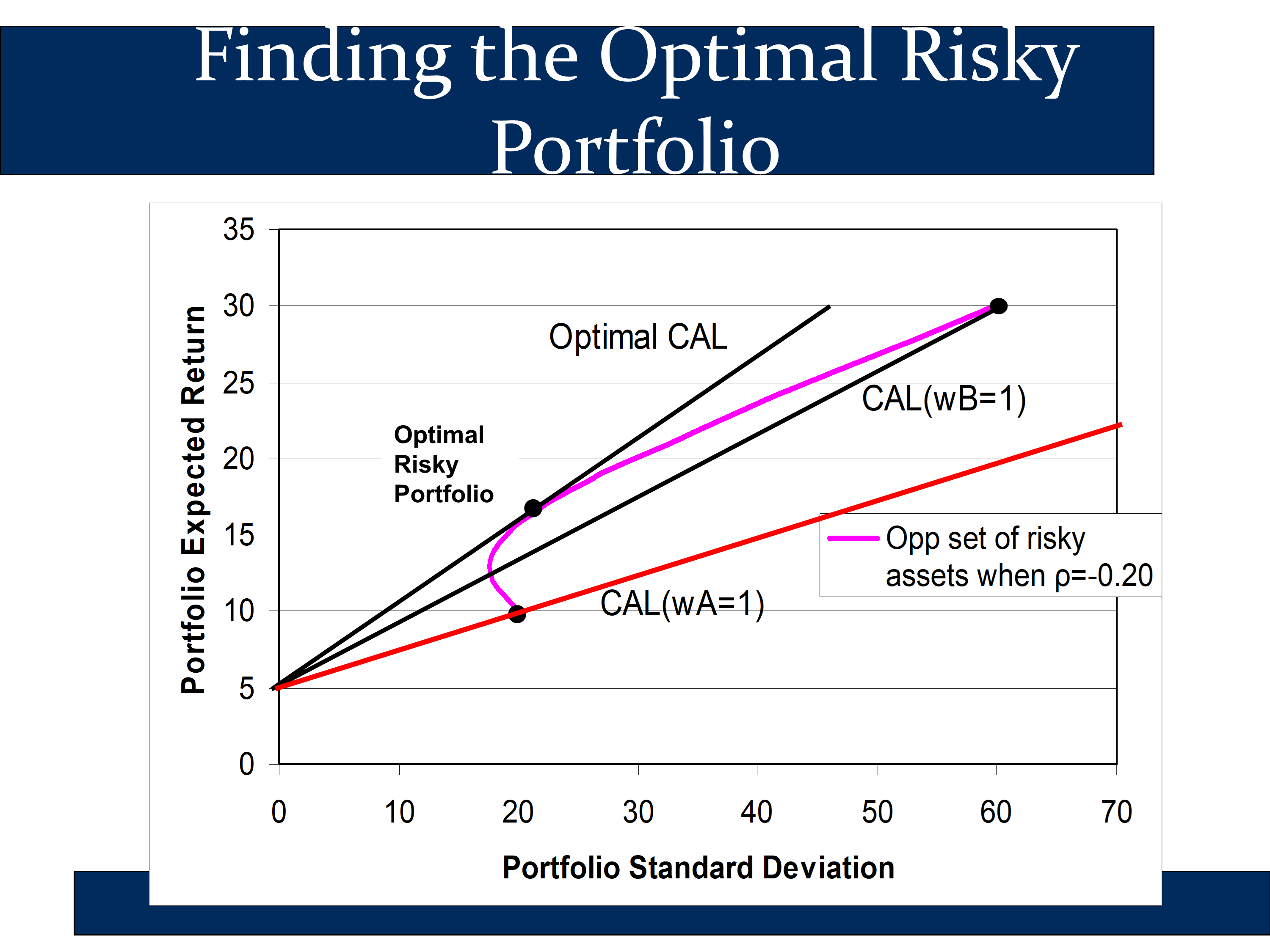
To find this risky portfolio, we plot out all points on the curved line and choose the one with the highest Sharpe ratio. To plot each point, we’ll need formulas for $E(r)$ and $σ$. We’ll show these in the following section.

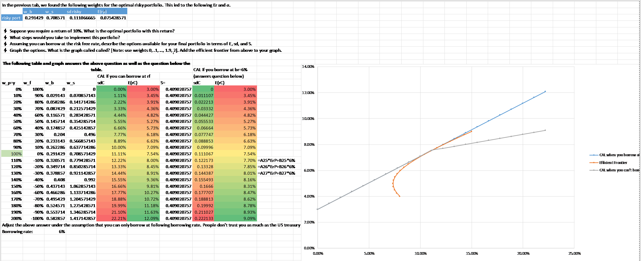
The full process of finding the optimal risky portfolio is illustrated below in Excel:

Modern Portfolio Theory

🙋How do you determine which specific various weighted combinations to include when calculating the optimal risky portfolio?(“Step 1”) Would these be the points that make up the minimum variance frontier?

See answer

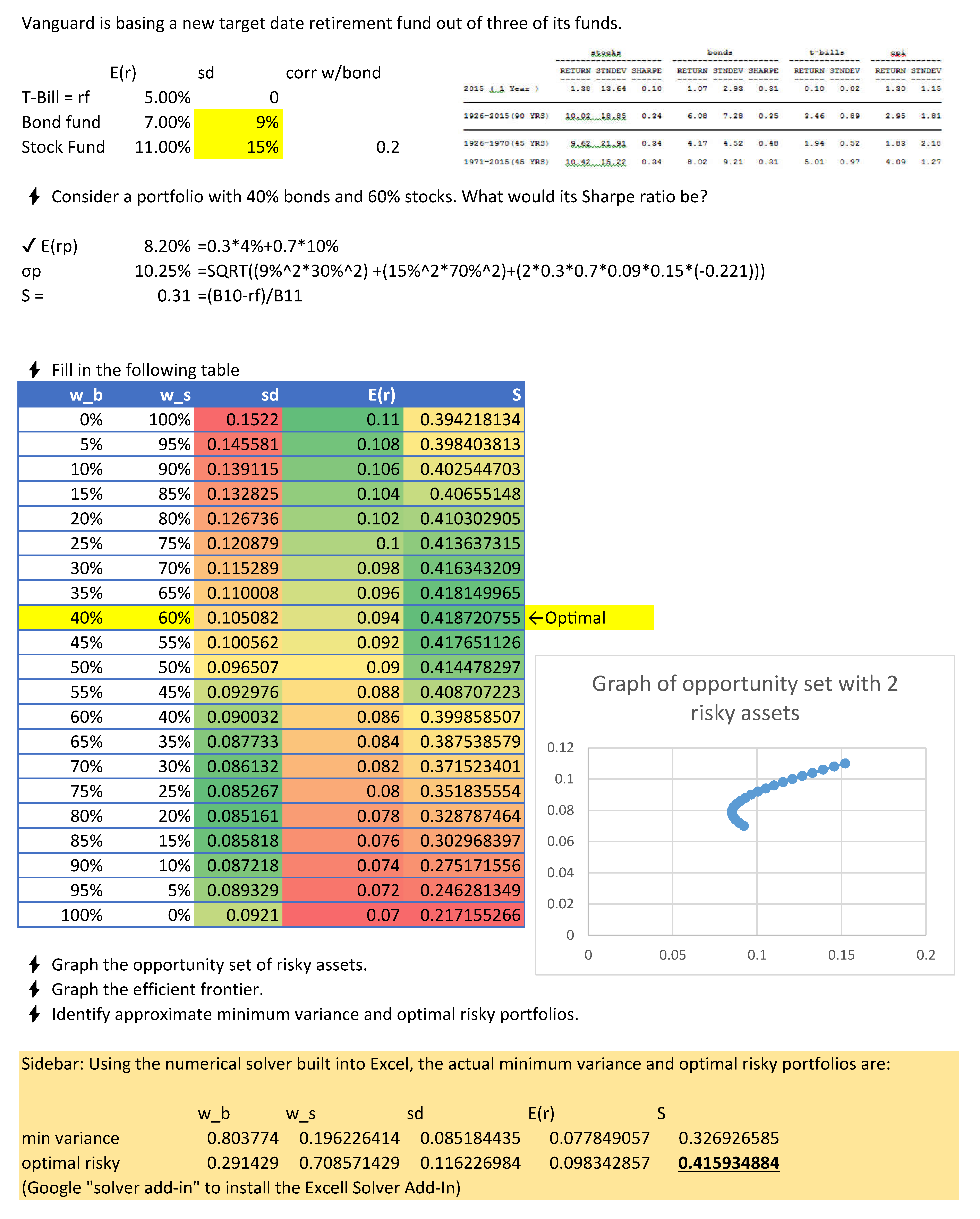
You want to include enough points that you can get very close to the truly optimal portfolio. However, there is no scientifically best approach. At the bottom of the spreadsheet, I use a computer optimization program for this to find an optimal risky portfolio that is 29.1429% bonds and 70.8571% stocks. Here is a far better tool to use than Excel:
https://qontigo.com/products/axioma-portfolio-optimizer/

The key equations for $Er_P$ and $σ_P$

In the previous lecture, we talked about how investing is a tradeoff between risk $(σ)$ and return $(Er)$. We investigated this tradeoff as an investor allocated their assets between a risky $(r_P)$ and a risk-free $(r_F)$ asset. In this lecture, we extend the analysis. We consider how an investor can find the optimal risky portfolio to mix with the risk-free asset.

This involves another risk-return tradeoff, as we allocate between two (or more) risky assets. As before, we look at $E_r$ and $σ$. Our new formulas for them are:

$$E(r_p) = w_1E(r_1) + w_2E(r_2) + \cdots$$

$$\sigma_p = \sqrt{Var(r_p)}$$

where

$$Var(r_p) = w_1^2 \sigma_1^2 + w_2^2 \sigma_2^2 + 2w_1w_2 \sigma_1 \sigma_2 \rho_{1,2}$$

Note, ρ_1,2 refers to the correlation between asset 1 and asset 2. Also, if you’reg not given ρ_1,2 then you can use ρ_1,2 = σ_1σ_2Cov(r_1, r_2).

✏️Image you are making a portfolio out of three mutual funds:

	E(r)	sd
T-Bill fund = rf	2.4%	0
Bond fund	4%	9%
Stock Fund	10%	15%	ρ1,2=-0.221

Imagine a risky portfolio consisting of 60% stocks and 40% bonds. What are the expected return, variance, and standard deviation of this portfolio?

✔Let’s just decide that bonds are asset 1 and stocks are asset 2.

$$\begin{aligned} E(r_p) &= w_1E(r_1) + w_2E(r_2) +⋯ \\ &= 40\% × 4\% + 60\% × 10\% \\ &= 7.6\% \end{aligned}$$ $$Var(r_p) = \textcolor{green}{{w_1}^2{\sigma_1}^2} + \textcolor{red}{{w_2^2 \sigma_2^2}} + \textcolor{royalblue}{{2w_1w_2 \sigma_1 \sigma_2 \rho_{1,2}}} \\ = \textcolor{green}{40\%^2 × 9\%^2} + \textcolor{red}{60\%^2 × 15\%^2} + \textcolor{royalblue}{2 × 40\% × 60\% × 9\% × 15\% × (-0.221)} \\ = 0.00796$$

$$\begin{aligned} \sigma_p &= \sqrt{Var(r_p)} \\ &= 0.00796^{\frac{1}{2}} \\ &\text{(enter this as 0.00796\textasciicircum .5)} \\ &= 0.08922 \\ &= 8.92\% \end{aligned}$$

🧭 Key insight:
It turns out that these new formulas are derived from the same classical formulas from probability that last week’s key formulas are derived from:

2 Pairs of Statistics & 4 Helper Formulas

Expected Value of Return:
CAL:
 $E(r_C) = r_F + y(E(r_P) - r_F)$
Two risky assets:
 $E(r_p) = w_1E(r1) + w_2E\,(r_2)$
Classic equation:
 $E(aX + bY) = a\,E(X) + b\,E(Y)$

Standard Deviation of Return (Risk):
CAL:
 $σ_C = y \;σ_P$
Two risky assets:
 $σ_P = SQRT({σ_1}^2\,{w_1}^2 + {σ_2}^2\,{w_2}^2 + 2\,w_1\,w_2\,Cov_{1,2})$
 $σ_P = SQRT({σ_1}^2\,{w_1}^2 + {σ_2}^2\,{w_2}^2 + 2\,w_1\,w_2\,σ_1\,σ_2\,Corr_{1,2})$
Classic equation:
 $Var(aX + bY) = a^2\,Var(X) + b^2\,Var(Y) + 2\,a\,b\,Cov(X,Y)$
* I wouldn't worry about using the two classic equations - but it's good to know the formulas Bruce used to come up with our equations.

Probability Helper Formulas:
Variance and Standard Deviation:
  $σ = \sqrt{Var}\quad\text{ and }\quad Var = σ^2$
Covariance and Correlation:
 $ρ_{12}=\frac{Cov(r_1,r_2)}{σ_1σ_2}\quad\text{ and }$
$\quad Cov(r_1,r_2)=ρ_{12}σ_1σ_2$

I prefer the risk equations that use standard deviation rather than variance and that use correlation rather than covariance:

• Standard deviation is measured in percentage points like returns are, so it’s easy to interpret.
• Correlation is always between -1 and 1, so it’s also easy to interpret.

✏️ Redo the last question, but imagine that instead of being told the standard deviation of the risky assets, you were told the variances. In particular the variance of the bond fund is .0081 and the variance of the stock fund is .0225.

Click/tap for Lecture 1 Formulas

Name

Equation

Example

Expected Return, $E(r_C)$

$E(r_C) = r_F + y (E(r_P)-r_F)$
or
$E(r_C) = y E(r_P) + (1-y) r_F$

= .04 + .50*(.12-.04) = .08 or 8%
or
= (.12 * .50) + (.04 * .50) = 8%

Standard Deviation of Complete Port, $σ_c$

$σ_c = y σ_p$

= .20 * .50 = .10 or 10%

Variance, $Var$

$Var = σ^2$ = σ^2

Var = 12%^2 = .0144

Standard Deviation, $σ$

$σ = \sqrt{Var} = Var^{\frac{1}{2}}$

σ = .0144^.5 = 12%

Risk Premium

Risk Premium $= E(r_C)-r_F$

= 12% - 2% = 10%

Sharpe Ratio, $S$

$S = \frac{E(r)-r_F}{σ}$

= (.12-.04)/.20 = (8/20) = .40

Equation for CAL

$E(r_C) = r_F + \frac{E(r_P) - r_F}{σ_P}σ_C$

Sharpe ratio = .8
E(r_C) = r_F + Sσ_C = 2% + .8 * 15% = 14%

Notation

$r_F$ = Return of Risk Free Assets

$r_P$ = Return of Portfolio of Risky Assets

$r_C$ = Return of Complete Portfolio

$E(r_P) / E(r_C)$ = Expected Return of Risky/Complete Portfolio

Occasionally I use $Er_P/Er_C$ as shorthand for $E(r_P)/E(r_C)$

$y$ = % of Portfolio in Risky Assets

$1-y$ = % in Risk-Free Assets

$σ/σ_P/σ_C$ = Standard Deviation

$S$ = Sharpe Ratio

Variance = Standard Deviation^2

Standard Deviation = SQRT of Variance

→ Complete formula page

✔Here, we just convert the variance to standard deviation and then just redo the problem as before. To convert between σ and Var, we use the following formulas:

$$\begin{aligned} Var &= \sigma^2 \text{, so} \\ σ &=\sqrt{Var} \end{aligned}$$

Therefore,

$$\begin{aligned} σ_1 &= .0081^.5 = 0.09 = 9\% \\ σ_2 &= .0225^.5 = 15\% \end{aligned}$$

Because these two standard deviations are identical to the standard deviations in the previous problem, we just do the exact same calculations and get the exact same answers.

$$\begin{aligned} E(r_p) &= w_1E\left(r_1 ) + w_2E(r_2 \right) +⋯ \\ &= 40\% × 4\% + 60\% × 10\% \\ &= 7.6\% \end{aligned}$$

$$Var(r_p) = \textcolor{green}{{w_1}^2 {σ_1}^2} + \textcolor{red}{{w_2}^2{σ_2}^2} + \textcolor{royalblue}{2w_1 w_2σ_1 σ_2 \rho_{1,2}} \\ \qquad= \textcolor{green}{40\%^2 × 9\%^2} + \textcolor{red}{60\%^2 × 15\%^2} + \textcolor{royalblue}{2 × 40\% × 60\% × 9\% × 15\%(-0.221)} \\ \qquad= 0.00796$$

$$\begin{aligned} σ_p &= \sqrt{Var(r_P)} \\ &= 0.00796^{\frac12} \\ &= \text{0.00796\textasciicircum.5 \quad (in Excel)} \\ &= 0.08922 \\ &= 8.92\% \end{aligned}$$

Clearly, these formulas are helpful and “not incredibly hard to use” once you get used to them. But you should be asking where they come from.

✏️ Consider the following data. What is the covariance between stocks and bonds?

	E(r)	sd
T-Bill fund = rf	2.4%	0
Bond fund	4%	9%
Stock Fund	10%	15%	ρ1,2=-0.221

✔The helper formulas we want are on this slide:

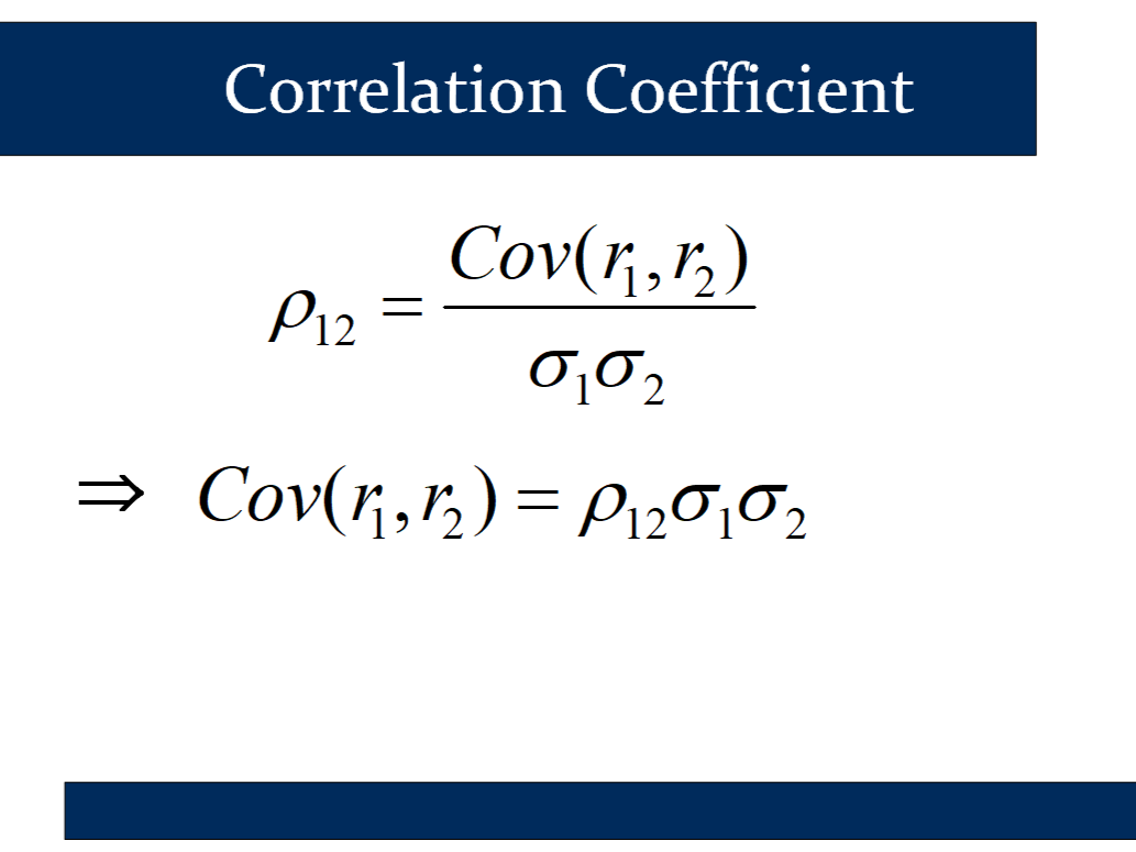
Cov(r_1, r_2) = ρ_1,2σ_1σ_2 = ρ_{1,2 *} σ_{1 *} σ_2 = -0.221 * 9% * 15% = -0.002984

✏️ In the above example, if the Covariance was .01, what would the correlation be?
✔ ρ_1,2 = (Cov r_1,r_2)/(σ_1*σ_2) = .01/(9% * 15% ) = .74

What if there are more than two assets?

The two formulas above can be used, as we saw, to build the optimal portfolio of risky assets when there are only two assets. But what if there are more than two assets?

In this case, there are more complicated formulas based on linear algebra (vectors and matrices). YOU ARE NOT RESPONSIBLE FOR THESE MORE COMPLICATED FORMULAS. But it’s nice to know that the material we’ve learned can be extended to optimize larger portfolios.

When you have six or more assets, you can use the extended formulas to calculate a “minimum variance frontier:“

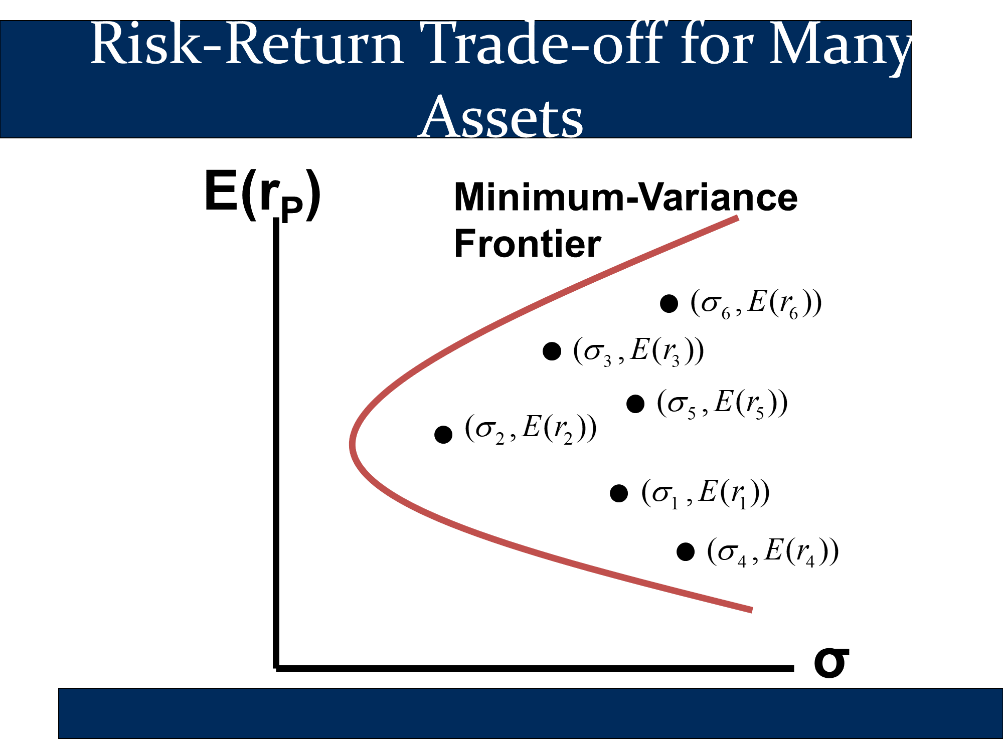
If you look at all of the portfolios you can construct with six assets and then plot their E(r_P) and σ_P, then you will get a cloud-like shape as above. If you isolate all portfolios that have the lowest possible variance for a specific expected return, you get the “minimum variance frontier.”

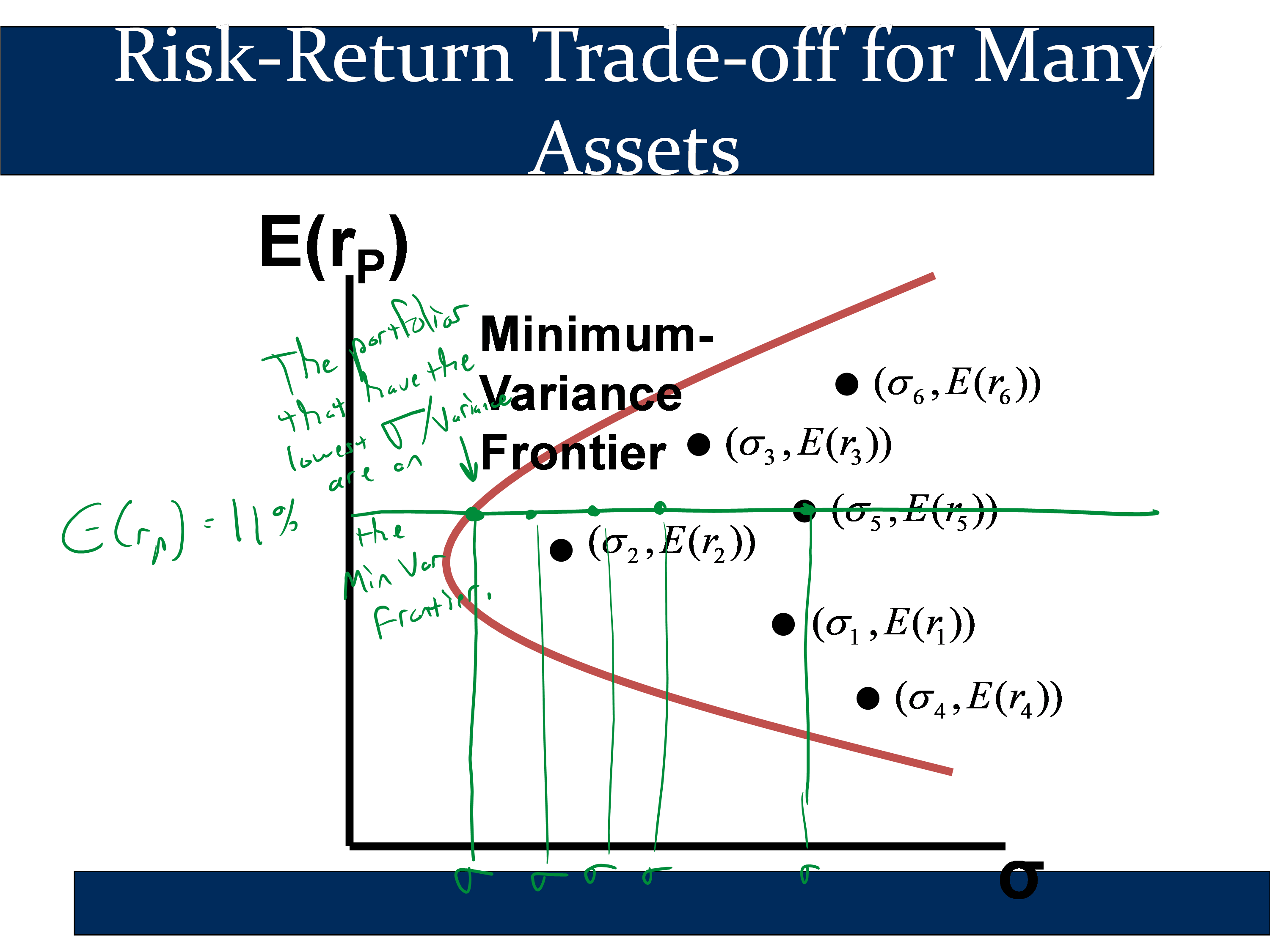
The portfolio with the lowest variance/sd of all portfolios made from those six assets is the “Global Minimum Variance” portfolio. If we throw away the portfolios that are beneath a better portfolio, we get the “Efficient Frontier,” which are the relatively “elite” portfolios that are left over.

The following graphic shows many example risky portfolios constructed as mixtures of the available securities. Note that the red dot portfolios cluster around the minimum variance frontier:

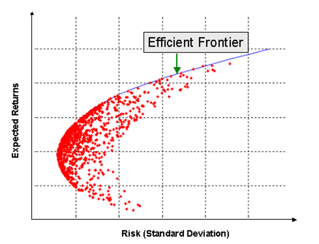
By choosing the portfolio in the efficient frontier with the highest Sharpe ratio, we get the optimal risky portfolio:

Using this, we can construct our CAL.

Build the CAL

Our end-goal is to find an optimal risky portfolio that we can use to build a Capital Allocation line. Then we can choose a complete portfolio from the CAL that matches our risk preferences.

To plot, just make a table with various values of y. For each value of y, you just apply our two main formulas for the CAL.

Formula
E(rC) = rF + y[E(rP) - rF]	σC = y σP

A far more complex example is illustrated here:

Modern Portfolio Theory

Risk preferences

✏️ An investor has the following utility function. Their coefficient of risk aversion, A, is 2.5 and their utility function is

$$U = E(r)- \frac{1}{2} A \sigma^2$$

Consider the following three portfolios. Which portfolio is best for this investor?

	1	2	3
y	10%	50%	110%
Erc	3.45%	5.27%	8%
σc	1.11%	5.55%	12.22%

✔

$$U = E(r) - .5 × 2.5 × σ^2$$ $$U_1 = 3.45\% - .5 × 2.5 × 1.11\%^2 = 0.0343 \text{ 🥉}$$ $$U_2 = 5.27\% - .5 × 2.5 × 5.55\%^2 = 0.0488 \text{ 🥈}$$ $$U_3 = 8\% - .5 × 2.5 × 12.22\%^2 = 0.0613 \text{ 🥇}$$

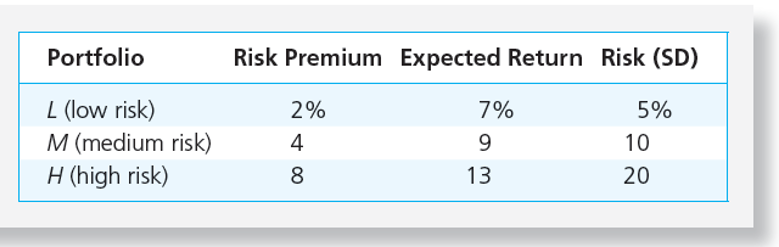
Suppose that there are three portfolios, L, M, and H:

Also, imagine there are three investors. Each investor has a different A.

In the following table each investor is represented by a row and each portfolio is represented by a column. In each cell, he’s put the utility of the portfolio for that specific investor. For example in the upper right, we have the utility of portfolio L for an investor with A=2.

$$U_L = E(r) - \frac{1}{2}A\sigma^2 = E(r) - .5 × A × σ^2 = .07 - .5 × 2.0 × .05^2 = 0.0675$$

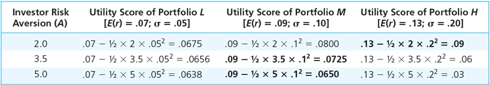
We can see from the table above that the first investor (A=2.0) will choose portfolio H. The second investor will choose portfolio M, and the third will choose portfolio M as well.

In the above example, the choice of optimal complete portfolio depends on the level of risk aversion. However, there are some portfolios that should never be chosen (regardless of risk aversion) because they are dominated by another portfolio.

Portfolio A dominates portfolio B if:

$$E(r_A) ≥ E(r_B)$$

and

$$σ_A ≤ σ_B$$

If a portfolio dominates the other, it is “better on both dimensions.” A dominated portfolio will never be chosen if the investor could, instead, choose the dominating portfolio.

✏️ Of the following four portfolios, which portfolio would never be chosen by any investor? (Hint: look for two portfolios where one portfolio dominates the other. Ie look for a pair of portfolios where one portfolio has a lower Er and a higher σ.)

1. $E(r_A)=9\% \quad σ_A= 10\%$
2. $E(r_B)= 11\% \quad σ_B= 12\%$
3. $E(r_C)= 7\% \quad σ_C= 9.9\%$
4. $E(r_D)= 8\% \quad σ_D= 11\%$

✔D is dominated by A because

• D has a lower expected return: ☹️E(rD)= 8% < E(rA)=9%🙂
• D has a higher risk: ☹️σ_D= 11% > σ_A= 10%🙂

✏️ The following table shows Er, σ and U for 11 portfolios on the same CAL. The bonus exercise below shows how we can determine that r_F = .07, E(r_P)=.150, and σ_P=.220, just by looking at the table. With some algebra, we can also find A=4.
Fill in the blank in the table. In other words, what is the utility when y=50%.

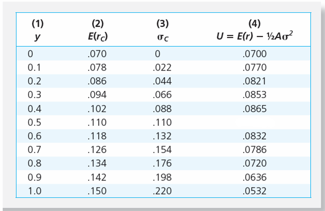
✔ When y=50%, $U = E(r) - \frac{1}{2}Aσ^2 = .110-.5× 4 × .110^2 = 0.0858$

🧠 This number is of a similar magnitude to the other utility numbers, so we can be confident in it!

Bonus exercise:

✏️ From what you know about the CAL, in the example above, what are r_F, E(r_P) and σ_P?

Hint: how does E(r_C) compare to E(r_P) when y=1?

✔ When y=100%, E(r_C)=E(r_P). The tables shows us that E(r_C) is .150 when y=1.0. Therefore, E(r_P)=.150.
Similarly, when y=100%, σ_C=σ_P . The tables shows us that σ_C is .220 when y=1.0. Therefore, σ_P=.220.
Finally, when y=0%, E(r_C) = r_F. The table shows us that E(r_C)= .070 when y=0, so r_F = .07.

Bonus exercise 2:

✏️ What is A?

Plug and chug: (help)

1. Equation:
   $$U = E(r)-.5Aσ^2$$
2. Plug:🔌
   

   Let’s look at when y = 1 and plug in: U = E(r)-.5Aσ^2

   $$.0532 = .150-.5A.220^2$$
3. Solve: 🚂
   $$.0532-.150 = -0.0968 = -.5A.220^2$$$$-0.0968 /(-.5)=0.1936 = A.220^2$$$$0.1936/(.220^2) = 4.0 = A$$
4. Reflect: 🧠
   

   The investor on that table has A=4.

In the following slide, he plots utility for each of the values in the table above:

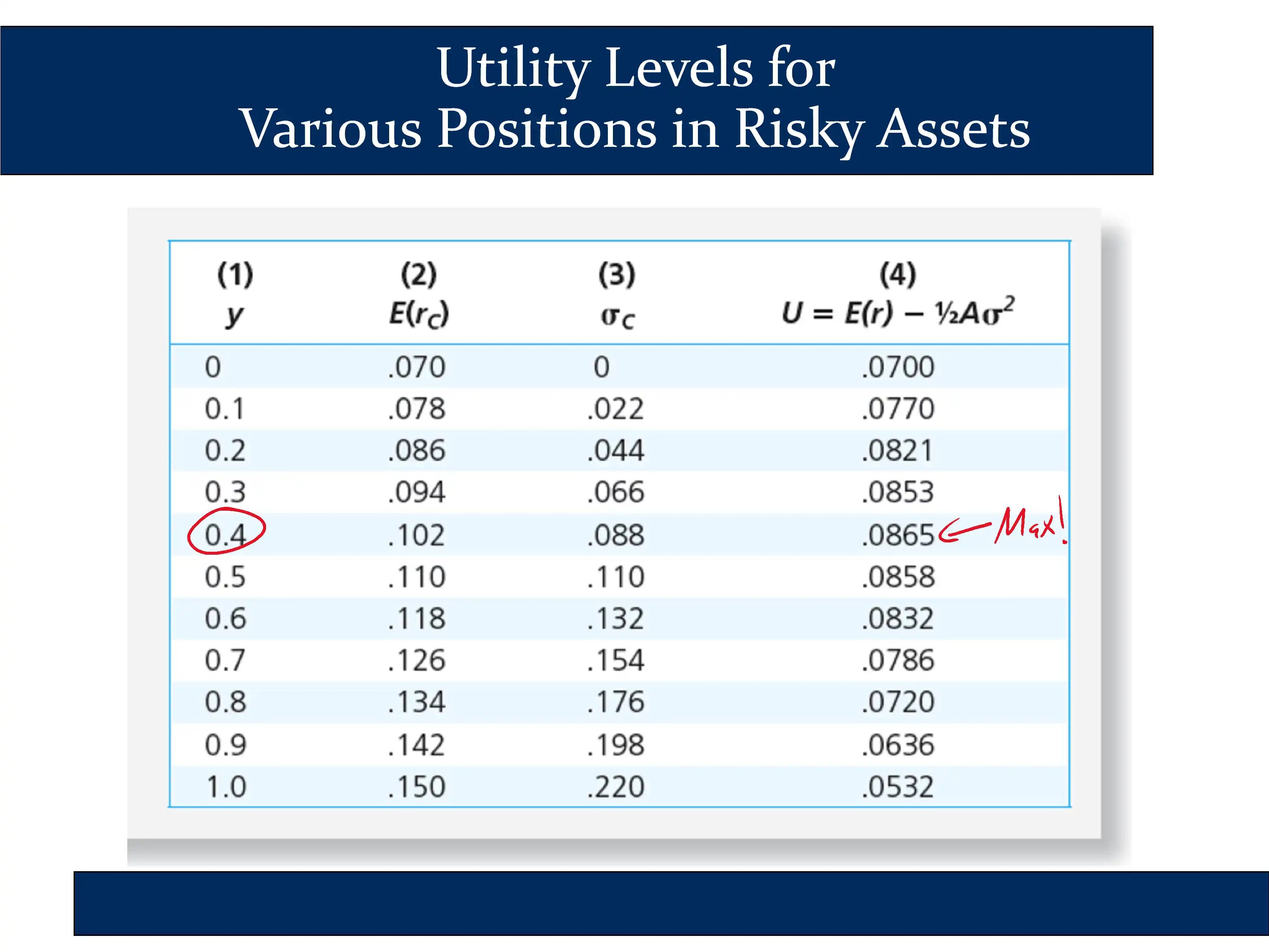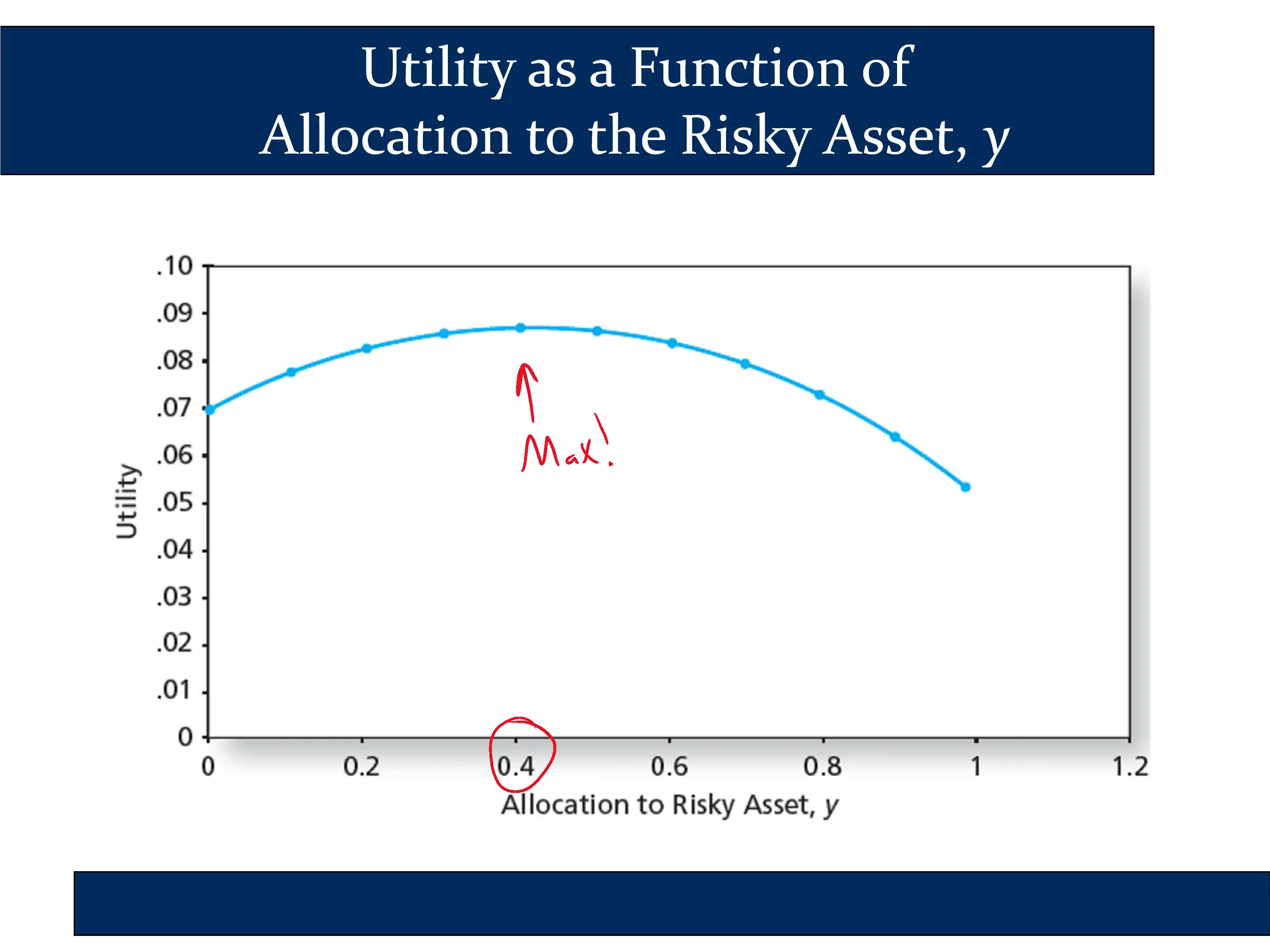The conclusion is that there is a specific point where utility is maximized. Looking at both the table and the chart, you can see that the utility is maximized around y=.4.

Therefore, for an investor with a risk aversion of A=4, the optimal capital allocation decision is for them to invest roughly 40% of their assets in the risky portfolio.

✏️ In the following diagram, what is the utility of portfolios A, B, C, D, and E?

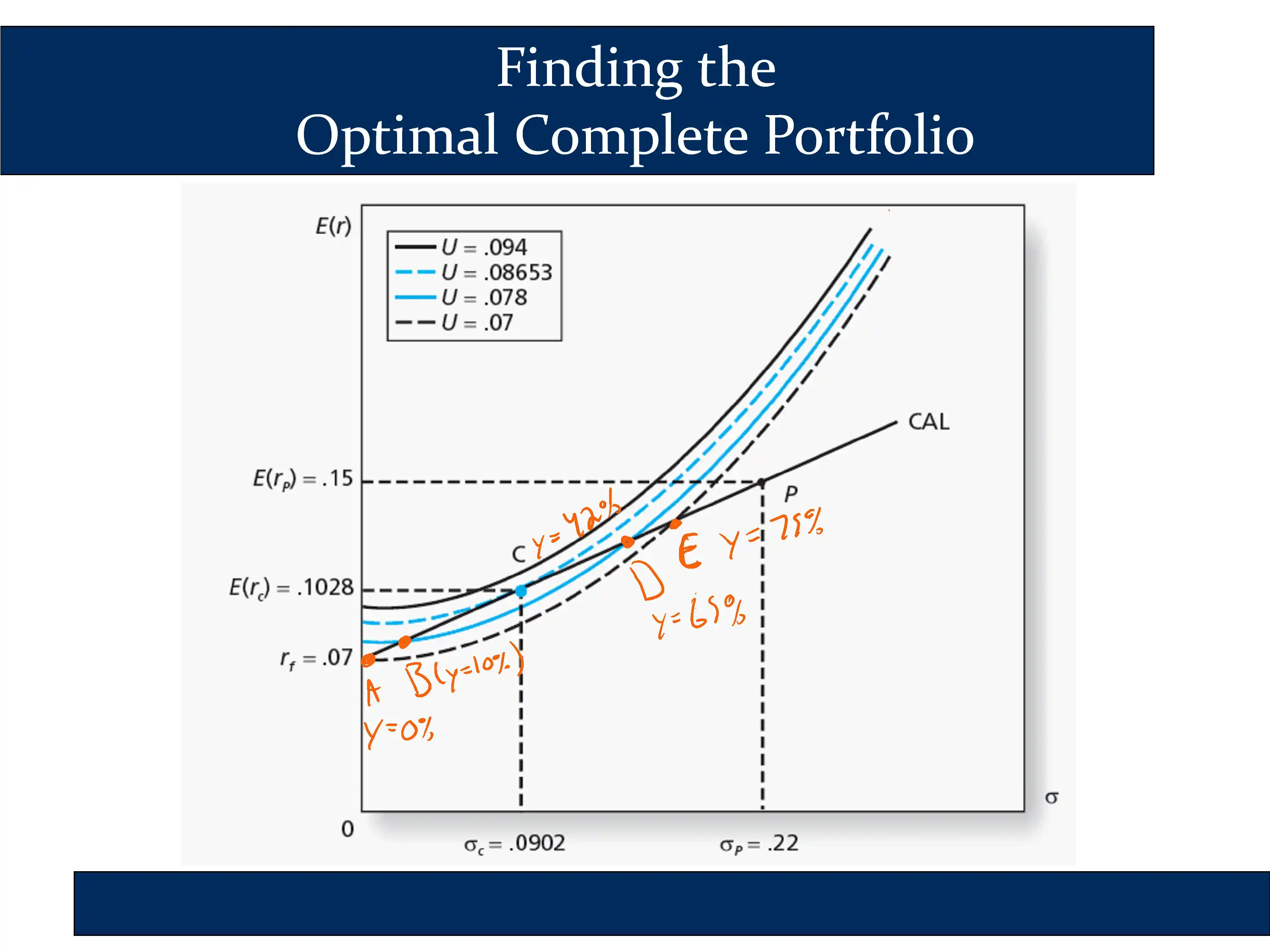
Portfolio A is on the dashed black line, so it receives a utility of .07.
Portfolio B is on the solid blue line, so it receives a utility of .078

✏️ If the values of y for each of the “lettered” portfolios is given on the diagram, what percentage of their assets should the investor allocate to risk assets?
✔ The highest utility is reached at portfolio C, so the investor should invest 42% of their investable wealth in risk assets.

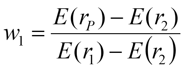
Using algebra/Plug and chug, (help) we could solve for the portfolio weights that will give us a specific Er in our risky portfolio.

…or we could just use the formula Bruce gave us:

✏️ Suppose you want to make a risky portfolio with an expected return of 7% out of the following two assets. What should you invest in each asset?

	E(r)	sd
Bond fund	4%	8%
Stock Fund	9%	15%

✔

$$\begin{aligned} w_1 &= \frac{E(r_P) - E(r_2)}{ E(r_1) - E(r_2)} \\ &= \frac{7\% - 9\%}{4\% - 9\%} \\ &= 40.0\% \end{aligned}$$

Plug and chug: (help)

1. Equation:
   

   Our main formula for Er in this lecture is: $E(r_p) = w_1E(r_1) + w_1E(r_1)$

2. Plug:🔌
   

   All of our money will either be invested in asset 1 or asset 2. Therefore, w_2 = 100%-w_1. If we substitute 100%-w_1 in for w_2, then we get:

   $$E(r_p) = w_1E(r_1) + (1 - w_1)\,E(r_2)$$
3. Solve: 🚂
   

   If we solve that equation for w_1 we get the formula Bruce gave us, above.