👨‍🏫 Notes

The previous two weeks, we studied the CAL and risky portfolio optimization. Together these are called Markowitz Portfolio optimization, Modern Portfolio Theory, or Mean-Variance Optimization.

Markowitz Portfolio theory takes the perspective of an investor, trying to find an optimal portfolio. It is like the demand curve for investments because it describes how investors will choose which securities to buy.

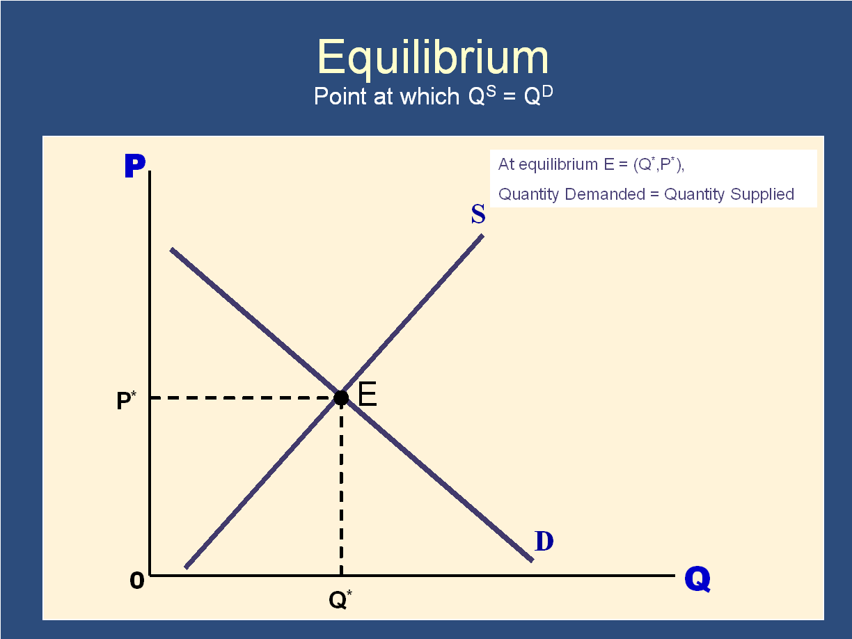
Could we upgrade our model by adding a supply curve. From economics, we know that Supply and Demand lead to a market equilibrium, which determines prices.

That’s terrific. If we add this concept of Supply and Demand to Markowitz Portfolio Optimization, we will get a theory of Asset Pricing. Specifically, we get the “Capital Asset Pricing Model.”

In summary:

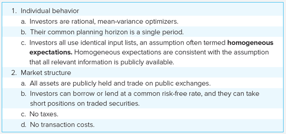
Markowitz Portfolio Optimization ➕ Supply & Demand = CAPM

Put another way, the CAPM is what you get when you assume that all investors are mean-variance optimizers and they all share the same beliefs and a couple other assumptions required to make the math work out.

↑ This is what Sharpe, Lintner, etc. did.

In the CAPM, the future cash flows of any given security are random, but they don’t depend on the prices of the securities. Therefore, we can think of these securities much like bonds - they have fixed random payoffs in the future. As we know from bonds, prices and rates of return are more or less interchangeable when you know the future cash payoffs. For example, if you are given the yield for a specific bond, you can easily calculate it’s price. Likewise, if you know the price of a bond, a computer can calculate it’s yield. In the CAPM, we do the same thing:

  Supply and demand together determine securities prices
  The securities prices and their fixed random payoffs determine the securities’ Expected return.

The final expected return is given by:

$$E(r_S)=r_F+β(E(r_M)-r_F)$$

You are likely very familiar with the above equation. These introductory remarks explain the logical steps that are taken to arrive at that equation.

In this model, everyone is selfishly optimizing their own interests:

  Firms and governments have already optimized and have decided which securities to issue. This is the supply of securities, and the model takes it as fixed.
  Investors optimize their holding by following Markowitz Portfolio Optimization (the tools we covered in the last two lectures).

Economists generally assume that prices will be set such that the quantity of securities demanded by investors equals the quantity supplied by the issuing firms and governments:

In summary:

Markowitz Portfolio Optimization ➕ Supply & Demand = CAPM

Assumptions

Outcome of investor’s optimal portfolio choice (Demand)

Recall that Markowitz Portfolio Optimization (aka Mean-Variance) can be divided into three steps.

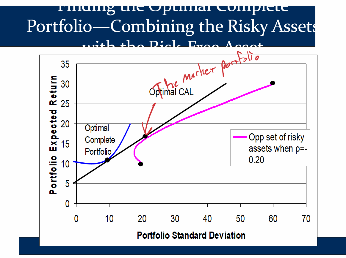
1.) Find the optimal risky portfolio. 2.) Construct the CAL. 3.) Choose the point on the CAL that balances risk and reward based on their individual preferences.

Regarding the first step, if all investors are looking at the same assets and have the same beliefs, they will all use the same inputs when finding the optimal risky portfolio (ie the same $E(r)$, $σ$, and $ρ$). Because, as we’ve seen, finding the optimal risky portfolio is a completely mechanical process, EVERY investor will have the same risky portfolio.

In contrast, different investors, may make different capital allocation decisions (CAL) based on their risk preferences. In other words, they may choose to hold different proportions of the risk free asset and their optimal risky portfolio.

Later on, when we combine supply and demand for securities, we will find that the optimal risky portfolio that every investor settles on $(r_P)$ is identical to the market portfolio. In other words, everyone buys every security in proportion to its market cap. In other words, every investor is an indexer and we all buy the most global market-cap-weighted index of all possible securities.

This leads us to the Mutual Fund Theorem:

• If all investors freely choose to hold a common risky portfolio identical to the market portfolio, they would not object if all stocks in the market were replaced with shares of a single mutual fund holding that market portfolio
• Implication: A passive investor may view the market index as a reasonable first approximation of an efficient risky portfolio. When I took Bodie’s doctoral seminar in finance, it was palpable how excited he was about the idea of financial engineering - that we could engineer products that would be ideal for individual investors. In hindsight, this looks a lot like target date retirement funds.

Supply and Demand for securities

Here is where we conclude that all investors will hold the market portfolio:

If all investors are holding the same optimal risk portfolio, and if Microeconomics 101 says that the supply of securities must equal the demand for securities, which securities must all investors demand? (If supply is going to equal demand)

For example, if Nikola wasn’t in the optimal risky portfolio, then supply would not equal demand! There would be a surplus.

What happens to the price if no one wants to own shares of FTX exchange? The price will drop until the quantity supplied equals the quantity demanded: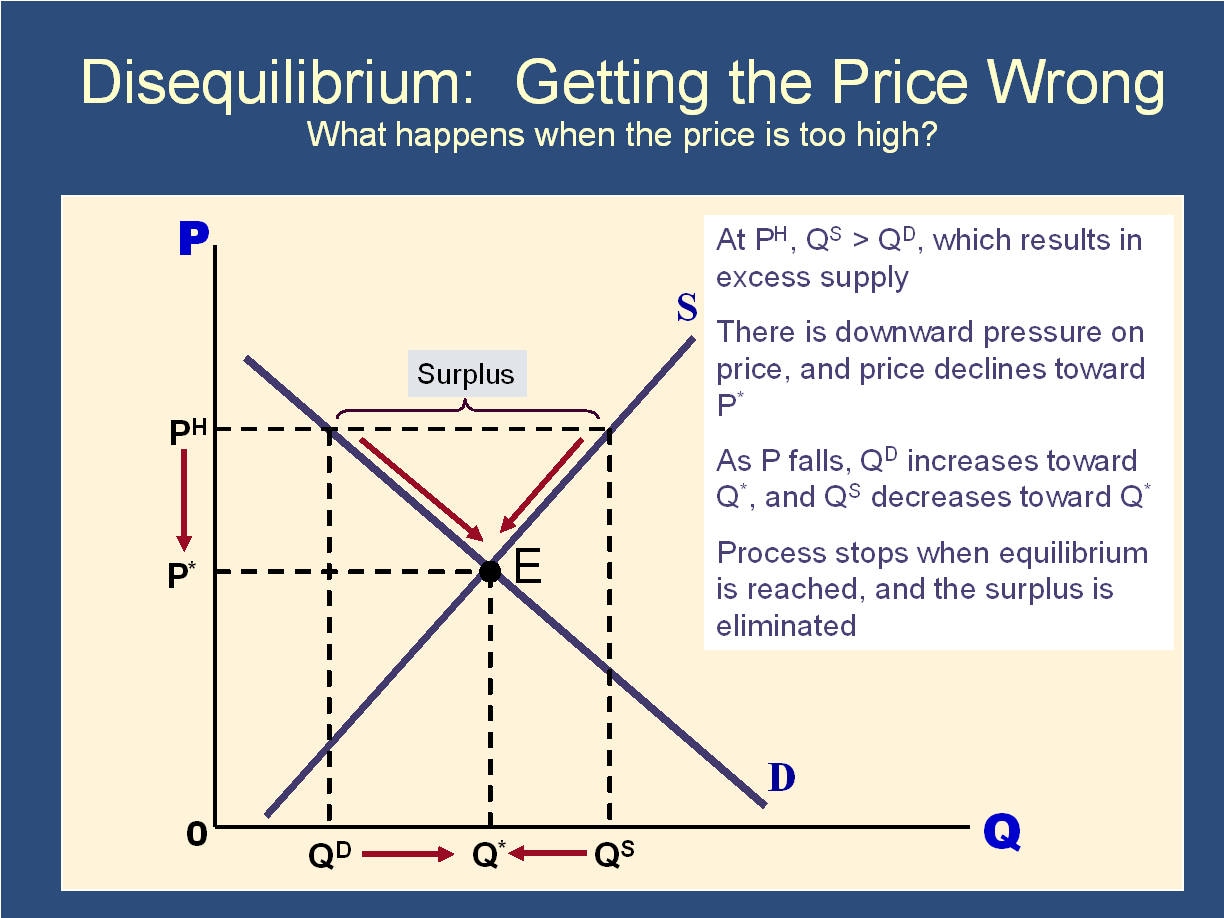

What happens to the price if people want to own more shares of TSLA than have actually been issued?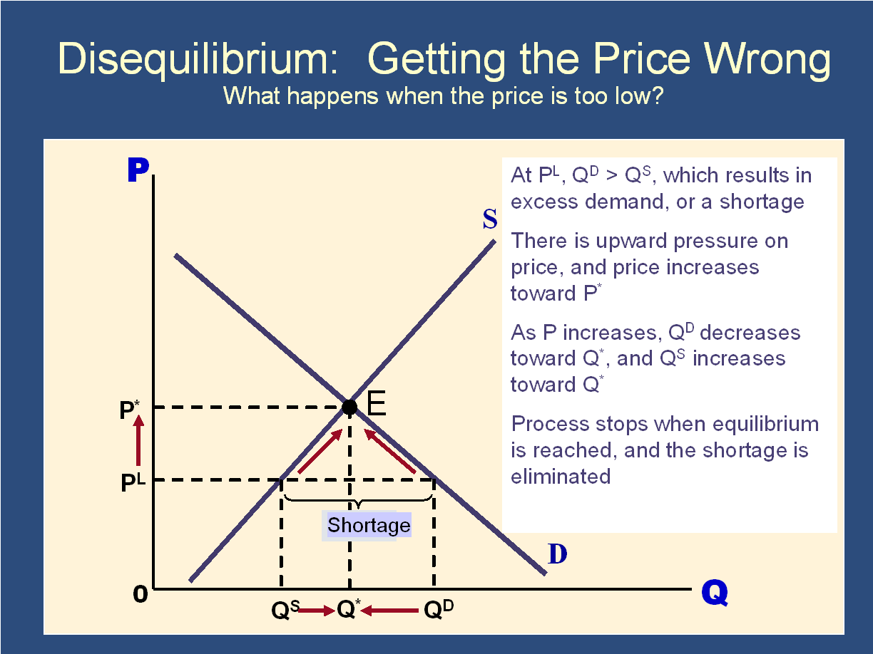

The only way that someone will hold every single security in the “universe of all securities” is if the price of FTX drops and the price of TSLA rises until everyone wants to own a little bit of each (in proportion to the number of shares each have issued).

In other words, prices will adjust until everyone owns the market portfolio.

If everyone has the same portfolio, and if every security must be owned by someone, then everyone must own every security. In other words, everyone must be indexers. This is why we could say above that “the optimal risky portfolio that every investor settles on $(r_P)$ is identical to the market portfolio.”

🙋 What happens when there is a surplus?

See answer

✔ Prices drop!

What happens to Nikola’s $E(r_N)$ when it’s price drops? It rises! Suddenly, it will become more attractive.

Bottom line: the price of Nikola will drop until it becomes part of everyone’s optimal risk portfolio.

That is how you add Supply and Demand to CAPM. The price of EVERY SECURITY drops (or rises) until it becomes part of the optimal risky portfolio (for everyone) and finally, investors are willing to hold all of the shares.

Because this happens for every security, every investor ends up holding every security. In other words, we all own index funds.

What we have just shown is that when everyone does their portfolio optimization, they get this:

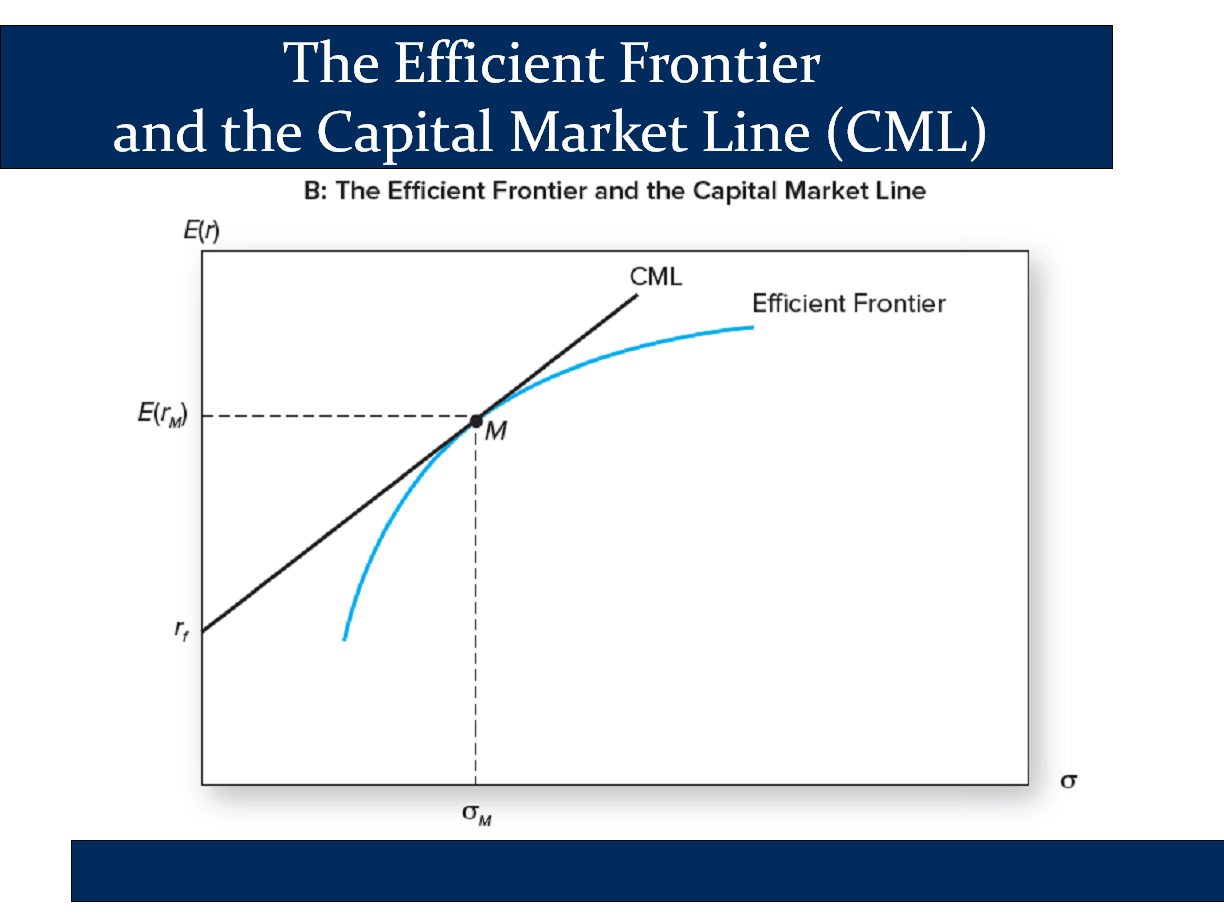
Because everyone has the market portfolio as their optimal risky portfolio, they all have the same CAL. People only differ in terms of the proportion of risky and risk-free assets that they hold in their portfolios (ie y), based on their risk aversion. For example, people closer to retirement will hold less risky assets and more risk-free free (ie they will be lower down on the CAL).

Because every investor has the same CAL and because the risky portfolio is the market portfolio, we rename the CAL to the CML (Capital Market Line):

What about securities prices and the key equation?

Above we established that everyone held the same optimal risky portfolio: the market portfolio.

What will be required for this to happen?

Basically, the most risky stocks must be cheap enough, so that when you calculate their Expected Returns, it compensates for the risk. In other words, the main determinant of expected return for each security must be the risk of that security:

$$E(r_S) = r_F + β(E(r_M)-r_F)$$

In other words, the way that we get investors to all hold the market portfolio is by pricing every security fairly and efficiently, such that everyone wants to hold every security for optimal diversification. In other words, prices of each security are set such that the risk premium of each security is proportional to the risk it adds.

There is a lot of truth in this! Most people in the real world will hold a vast universe of securities because of the diversification benefits that this provides. They are willing to hold them all because they can’t identify some securities that are better deals that others (ie EMH). In other words we all, more or less, consider most stocks to be fairly priced in comparison to other stocks (at least we don’t think we can make any money off of mispricings). (Yeah… as I said before, the CAPM is, at best, just an approximation.)

How is the Market Risk Premium determined?

The next result that comes out of the math of the CAPM is that it tells us how the market risk premium is decided:

• The risk premium on the market portfolio will be proportional to its risk and the degree of risk aversion of the average investor:

$$E(R_M) = Aσ^2_M*$$

Where $σ^2_M$ is the variance of the market portfolio and $A$ is the average degree of risk aversion across investors.

I also find this fairly compelling. Because we are integrating supply and demand, it can give us some insights into how market returns are determined. This gives us some insight as to why stock market returns will tend to be around 8%-15%.

Return and Risk For Individual Securities

Above, we said that
  the way that we get investors to all hold the market portfolio is by pricing every security fairly and efficiently, such that everyone wants to hold every security…. In other words, prices of each security are set such that the risk premium of each security is proportional to the risk it adds.

We can see this by rearranging our core equation, bringing $r_F$ to the left. In this version, instead of telling us the Expected Return for S, it tells us the Risk Premium for S. In this form, we can see that the Risk Premium for S is proportional to β:

$$E(r_S) = r_F + β(E(r_M)-r_F)$$

    ↑↑↑↑↑↑↑↑↑ On the left, we have the risk premium of the security in question
      ↑ this says that the risk premium of the security is proportional to β.

Basically, the expected return demanded by the market for a given security is proportion to β. Beta represents the risk that a given security adds to someone’s portfolio when that person is already investing in the entire market portfolio.

Bruce puts this as follows:

• The risk premium on individual securities, $E(r_S)-r_F$, is a function of the individual security’s contribution to the risk of the market portfolio.

$$E(r_S) - r_F = β(E(r_M)-r_F)$$

• An individual security’s risk premium is a function of β, which is determined by the covariance between the security’s returns and the market portfolio.

In that second bullet point, he is referring to the formula β. You aren’t responsible for this, but beta can be calculated as follows

$$β_i=\frac{Cov_{(r_M,r_i)}}{σ_M σ_i} = \frac{σ_i}{σ_M}^ρ_(M,i)$$

In other words, as he says, “β is determined by the covariance between the security’s returns and the market portfolio.”